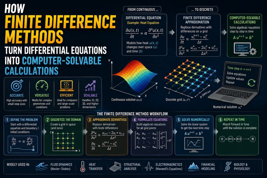

Many of the laws used in science and engineering are written as differential equations. These equations describe how physical quantities change with position, time, or both. They appear in models of heat flow, fluid motion, structural deformation, electrical circuits, chemical diffusion, population growth, weather, and countless other systems. 🌡️🌊⚙️
The difficulty is that many differential equations cannot be solved exactly with a neat mathematical formula.
Computers, meanwhile, do not naturally manipulate continuous derivatives in the same way mathematicians do on paper. A computer works with finite numbers stored at discrete locations.
Finite difference methods, or FDM, bridge these two worlds.
They replace derivatives with approximate arithmetic expressions involving values at nearby points. Once this transformation is performed, a differential equation becomes a collection of ordinary algebraic calculations that a computer can solve.
The central idea is simple:
Instead of asking exactly how a function changes at every possible point, sample the function at many closely spaced points and estimate the derivatives from the differences between those values. 💻📐
This approach has become one of the foundational techniques of numerical analysis and computational engineering.
📘 What Is a Differential Equation?
A differential equation is an equation involving one or more derivatives of an unknown function.
A simple example is:
dy/dx = 2x
This equation says that the rate at which y changes with respect to x is equal to 2x.
In this particular case, calculus gives an exact solution:
y = x² + C
But many real problems are much more complicated.
Consider the heat equation:
∂T/∂t = α ∂²T/∂x²
Here:
T represents temperature,
t represents time,
x represents position,
and α is a thermal diffusivity constant.
This equation describes how heat spreads through a material. 🌡️
For simple geometries and boundary conditions, analytical solutions may exist. But if the geometry, materials, or boundary conditions become complicated, exact solutions can become extremely difficult or impossible to obtain.
That is where numerical methods become essential.
🔢 Computers Prefer Discrete Numbers
Mathematical models often describe a continuous world.
A metal rod, for example, contains temperature values at every possible point along its length.
A mathematical function might represent this as:
T(x)
for every real value of x.
A computer cannot store infinitely many values.
Instead, engineers divide the domain into a finite set of points called a grid or mesh.
Suppose a rod is 1 meter long.
Instead of representing temperature continuously, we might calculate it at:
x = 0.0, 0.1, 0.2, 0.3, …, 1.0 meters
These points are called grid points or nodes.
The distance between neighboring points is often represented by:
Δx
or simply:
h
If the spacing is 0.1 meters:
h = 0.1
Now the computer only needs to store temperature at these discrete positions.
📐 From Derivatives to Differences
A derivative measures how quickly a function changes.
For a function f(x), the derivative is formally defined using a limit:
f′(x) = lim[h→0] (f(x+h) – f(x))/h
A finite difference method takes inspiration from this expression but does not let h become infinitely small.
Instead, it chooses a small finite spacing.
So the derivative can be approximated as:
f′(x) ≈ [f(x+h) – f(x)] / h
This is called a forward difference approximation.
Instead of calculating an abstract derivative, the computer performs:
- subtraction,
- division.
Those are simple numerical operations. 🧮
This is the key transformation that makes finite difference methods work.
➡️ Forward Difference
Suppose we know:
f(x)
and:
f(x+h)
Then:
f′(x) ≈ [f(x+h) – f(x)] / h
This approximation uses the current point and the next point.
For example, suppose:
f(2) = 4
and:
f(2.1) = 4.41
Then:
f′(2) ≈ (4.41 – 4) / 0.1
which gives:
4.1
For f(x) = x², the exact derivative is:
f′(x) = 2x
so at x = 2, the exact value is:
4
The approximation gives 4.1.
It is close, but not exact.
The difference is called numerical error.
⬅️ Backward Difference
Another approximation uses the current point and the previous point:
f′(x) ≈ [f(x) – f(x-h)] / h
This is called a backward difference.
Forward and backward differences are useful in different situations, especially when values are only available on one side of a point.
For example, near the edge of a computational domain, engineers may not have data beyond the boundary.
A one-sided difference can then be convenient.
↔️ Central Difference
A more accurate approximation often uses points on both sides:
f′(x) ≈ [f(x+h) – f(x-h)] / 2h
This is called a central difference.
Because it balances information from both directions, the errors tend to cancel more effectively.
Central differences are widely used in numerical simulations.
They often provide better accuracy than simple forward or backward differences for the same grid spacing. 🎯
🧱 Approximating Second Derivatives
Many important differential equations involve second derivatives.
For example:
d²f/dx²
A common finite difference approximation is:
d²f/dx² ≈ [f(x+h) – 2f(x) + f(x-h)] / h²
This expression appears constantly in computational physics and engineering.
It is especially important for equations describing:
🌡️ heat conduction
🎸 vibrations
🌊 waves
⚡ electrostatic potential
🧪 diffusion
Instead of calculating the second derivative directly, the computer combines values from three neighboring grid points.
🌡️ Example: Heat Flow Through a Rod
Imagine a metal rod whose left end is held at:
100°C
and whose right end is held at:
0°C
We want to know the steady-state temperature inside the rod.
For simple one-dimensional steady heat conduction, the governing equation can be:
d²T/dx² = 0
Using the finite difference approximation:
(Tᵢ₊₁ – 2Tᵢ + Tᵢ₋₁) / h² = 0
Multiplying by h² gives:
Tᵢ₊₁ – 2Tᵢ + Tᵢ₋₁ = 0
Rearranging:
Tᵢ = (Tᵢ₋₁ + Tᵢ₊₁) / 2
This result has a very intuitive meaning.
At steady state, the temperature at each interior point is approximately the average of the temperatures at its neighboring points.
The original differential equation has now become an algebraic relationship. 💡
That is exactly what a computer needs.
🧮 Building a System of Equations
Suppose the rod is divided into five interior points.
We may have unknown temperatures:
T₁, T₂, T₃, T₄, T₅
At each point, the finite difference approximation generates one equation.
For example:
-2T₁ + T₂ = -100
T₁ – 2T₂ + T₃ = 0
T₂ – 2T₃ + T₄ = 0
and so on.
Together, these form a system of linear equations.
In matrix form, engineers write:
A T = b
where:
A is a matrix of coefficients,
T contains the unknown temperatures,
and b contains known boundary information.
Computers are extremely good at solving systems like this.
Thus, a continuous differential equation has been transformed into linear algebra. 🔢➡️💻
⏱️ Time-Dependent Problems
Many physical systems change over time.
Consider the heat equation again:
∂T/∂t = α ∂²T/∂x²
Now we must discretize both:
📍 space
⏱️ time
Suppose:
Δx is the spatial grid spacing
and:
Δt is the time step.
The time derivative can be approximated using:
(Tᵢⁿ⁺¹ – Tᵢⁿ) / Δt
where:
i identifies position,
and:
n identifies the current time step.
The spatial second derivative can be approximated by:
(Tᵢ₊₁ⁿ – 2Tᵢⁿ + Tᵢ₋₁ⁿ) / Δx²
Substituting these expressions into the heat equation gives:
(Tᵢⁿ⁺¹ – Tᵢⁿ)/Δt = α(Tᵢ₊₁ⁿ – 2Tᵢⁿ + Tᵢ₋₁ⁿ)/Δx²
Now the computer can calculate future temperatures from current values.
🚀 Explicit Finite Difference Methods
If the new solution at time n+1 can be calculated directly from already-known values at time n, the method is called explicit.
For the heat equation:
Tᵢⁿ⁺¹ = Tᵢⁿ + r(Tᵢ₊₁ⁿ – 2Tᵢⁿ + Tᵢ₋₁ⁿ)
where:
r = αΔt / Δx²
The computer can repeatedly apply this equation:
Current temperatures
⬇️
Calculate next time step
⬇️
Store new temperatures
⬇️
Repeat
Explicit methods are often straightforward and computationally inexpensive per step.
However, they can have strict stability limits.
🔒 What Is Numerical Stability?
A numerical algorithm is stable if small numerical errors do not grow uncontrollably as calculations proceed.
Consider an explicit heat-equation scheme.
If the time step is too large relative to the grid spacing, tiny rounding or approximation errors can grow dramatically.
Instead of a smooth temperature distribution, the simulation may begin producing oscillations or enormous meaningless values. 💥
For a simple one-dimensional heat equation, a stability condition often takes the form:
αΔt / Δx² ≤ 1/2
This means that reducing the spatial grid size may require reducing the time step as well.
Numerical stability is one of the most important ideas in computational mathematics.
A mathematically correct differential equation can still produce a useless simulation if the numerical method is unstable.
🧠 Implicit Finite Difference Methods
An alternative is an implicit method.
Implicit schemes use values from the new time level in the finite difference equations.
Instead of calculating each future value directly, the algorithm forms a system of equations that must be solved simultaneously.
This requires more computational work per time step.
However, implicit methods can often remain stable with much larger time steps.
The tradeoff is therefore:
Explicit methods: simpler steps, potentially smaller allowed time steps.
Implicit methods: more expensive steps, often better stability.
Engineers choose between them based on the application.
⚖️ Accuracy and Grid Spacing
Finite difference methods are approximations.
Their accuracy generally improves as the grid becomes finer.
If:
h = 0.1
produces one level of error, then using:
h = 0.01
may produce a much better approximation.
However, finer grids require more calculations.
In one dimension, reducing grid spacing by a factor of 10 may create roughly 10 times as many points.
In two dimensions, it may create roughly 100 times as many points.
In three dimensions, it may create roughly 1,000 times as many grid points. 📈
This creates one of the central tradeoffs in numerical simulation:
Accuracy vs. computational cost
🎯 Truncation Error
When a derivative is replaced by a finite difference expression, some information is discarded.
The resulting discrepancy is called truncation error.
For example, a forward difference approximation typically has error proportional to:
O(h)
A common central difference approximation has error proportional to:
O(h²)
This means that when h becomes smaller, the central difference error may decrease much more rapidly.
Higher-order finite difference formulas can achieve even greater accuracy by using more neighboring points.
💻 Round-Off Error
Making the grid extremely fine does not guarantee unlimited accuracy.
Computers represent numbers with finite precision.
Very small differences between nearly equal numbers can introduce round-off error.
For example:
f(x+h) – f(x)
may involve subtracting two almost identical floating-point numbers.
If h becomes excessively small, numerical precision can become a problem.
So engineers seek a practical balance between:
📉 truncation error
💻 round-off error
⏱️ computation time
💾 memory usage
🧱 Boundary Conditions
Differential equations generally require boundary conditions.
These specify what happens at the edges of the computational domain.
Common types include:
🌡️ Dirichlet Boundary Conditions
The value itself is specified.
For example:
T(0) = 100°C
🌬️ Neumann Boundary Conditions
A derivative is specified.
For example:
dT/dx = 0
which might represent an insulated boundary with no heat flow.
🔄 Mixed Boundary Conditions
A combination of the value and derivative may be specified.
Boundary conditions are essential because they determine which physical solution the differential equation represents.
Finite difference methods must approximate these boundary conditions carefully.
🌊 Finite Differences for Wave Equations
Wave behavior is also commonly modeled with differential equations.
A simplified wave equation is:
∂²u/∂t² = c² ∂²u/∂x²
where:
u might represent displacement,
and:
c is wave speed.
Finite difference approximations can turn this equation into calculations describing how the wave moves from one time step to the next.
Applications include:
🎸 vibrating strings
🌊 water waves
🔊 acoustics
🌍 seismic waves
📡 electromagnetic systems
A computer can simulate how disturbances propagate, reflect, and interact.
🧪 Diffusion and Chemical Transport
Chemical diffusion describes how molecules spread from high-concentration regions toward lower-concentration regions.
The governing equation often resembles the heat equation:
∂C/∂t = D ∂²C/∂x²
where:
C represents concentration,
and:
D is a diffusion coefficient.
Finite difference methods can simulate how substances move through:
🧪 chemical reactors
🧬 biological tissues
🌱 soil
💧 groundwater
🔋 battery materials
The same mathematical technique can therefore model very different physical phenomena.
⚡ Electromagnetics
Maxwell’s equations describe electricity and magnetism.
A famous computational method called the Finite-Difference Time-Domain method, or FDTD, uses finite differences to simulate electromagnetic waves.
FDTD can model:
📡 antennas
📶 wireless signals
🔦 optical devices
🛰️ radar systems
💻 high-speed electronic circuits
The electromagnetic field is evaluated at discrete points in space and updated through time.
This allows engineers to study how waves propagate through complicated environments.
🌦️ Weather and Fluid Flow
Fluid dynamics involves differential equations such as the Navier-Stokes equations.
These describe fluid velocity, pressure, density, and other quantities.
Atmospheric and ocean models divide large regions into computational grids.
At each grid point, numerical methods approximate changes in:
🌡️ temperature
💨 wind velocity
💧 humidity
🌊 pressure
☁️ other atmospheric quantities
Finite difference ideas have historically played a major role in computational fluid dynamics and weather prediction.
Modern simulation systems may combine finite differences with finite volume, spectral, and other numerical approaches.
🔧 Structural Engineering
Finite difference methods can also help solve equations describing deformation in structures.
Engineers may model quantities such as:
🏗️ beam deflection
⚙️ plate bending
📏 stress distributions
🌉 structural vibrations
For very complex geometries, the finite element method is often more convenient.
However, finite difference methods remain valuable when the geometry fits naturally onto a structured grid.
🆚 Finite Difference vs. Finite Element Methods
Finite difference methods are sometimes confused with finite element methods, or FEM.
Both convert continuous differential equations into computer-solvable systems, but they approach the problem differently.
Finite differences approximate derivatives directly at grid points.
Finite element methods divide the domain into small elements and approximate the solution using basis functions.
Finite difference methods are often:
✅ Simple to understand
✅ Efficient on rectangular structured grids
✅ Easy to implement for many standard equations
Finite element methods are often better suited for:
🔺 Complex geometries
🏗️ Irregular boundaries
🧱 Complicated material regions
The appropriate method depends on the problem.
🆚 Finite Difference vs. Finite Volume Methods
Another related method is the finite volume method.
Finite volume methods divide the domain into small control volumes and apply conservation laws to each one.
They are especially popular in computational fluid dynamics because they naturally conserve quantities such as:
⚖️ mass
⚡ energy
📦 momentum
Finite difference methods focus more directly on derivative approximations.
In some simple cases, the resulting equations can look very similar.
🖥️ Why Matrices Become So Important
When finite difference methods are applied to large problems, they often produce huge systems of equations.
A 3D simulation might contain millions of unknowns.
This leads to mathematical systems such as:
A x = b
The matrix A is often sparse, meaning most entries are zero.
Why?
Because each grid point usually interacts only with nearby neighbors.
For example, a point might depend only on:
⬅️ left neighbor
➡️ right neighbor
⬆️ upper neighbor
⬇️ lower neighbor
Sparse matrix algorithms exploit this structure to save both memory and computation.
This is why numerical linear algebra is so closely connected to finite difference simulation.
🚀 Parallel Computing
Large finite difference simulations are well suited to parallel computing.
If different regions of a grid can be updated independently for part of the calculation, many processor cores can work simultaneously.
Modern simulations may run on:
🧠 multicore CPUs
🎮 GPUs
⚡ supercomputers
☁️ computing clusters
Each processor handles part of the grid.
Neighboring processors exchange boundary data as required.
This allows scientists to solve problems involving millions or billions of grid cells.
📏 Grid Refinement
How can engineers know whether their simulation is accurate enough?
One common technique is grid refinement.
The same problem is solved using progressively smaller grid spacing.
For example:
h = 0.1
then:
h = 0.05
then:
h = 0.025
If the answers converge toward the same solution, confidence increases that the numerical approximation is accurate.
This process is known as a grid convergence study.
It is an important part of reliable computational modeling.
⚠️ Numerical Solutions Are Not Automatically Correct
A computer can produce thousands of decimal places, but that does not mean the answer is physically meaningful.
Numerical simulations can fail because of:
❌ Incorrect equations
❌ Poor boundary conditions
❌ Inadequate grid resolution
❌ Unstable time steps
❌ Programming errors
❌ Inaccurate physical parameters
Engineers therefore perform verification and validation.
Verification asks:
Did we solve the mathematical equations correctly?
Validation asks:
Do those equations accurately represent the real physical system?
Both are essential.
🧠 Why Finite Difference Methods Are So Powerful
The true power of finite differences comes from converting difficult calculus into repeated local arithmetic.
A derivative may look mathematically abstract:
∂²T/∂x²
but after discretization it becomes something like:
(Tᵢ₊₁ – 2Tᵢ + Tᵢ₋₁)/h²
A computer can evaluate this expression millions of times very efficiently.
By repeating these calculations over a grid, engineers approximate the behavior of an entire physical system.
The method transforms:
Continuous mathematics → discrete grid → algebraic equations → computer calculation 💻
🚀 The Future of Numerical Simulation
Finite difference techniques remain important even as computational science becomes more advanced.
Modern developments include:
🤖 AI-assisted simulation
🎮 GPU acceleration
⚡ adaptive numerical methods
☁️ cloud-based scientific computing
🧠 hybrid physics and machine-learning models
🏭 digital twins
A digital twin, for example, may continuously simulate a physical machine while sensor data updates the model in real time.
Finite difference and related numerical techniques can provide the physical foundation for such systems.
As computing power continues to increase, engineers can use finer grids, larger domains, and more realistic models.
🌟 Conclusion
Finite difference methods allow computers to solve differential equations by replacing continuous derivatives with numerical approximations based on neighboring values.
Instead of representing a physical variable at infinitely many points, the method divides space and time into discrete grids.
A derivative such as:
df/dx
becomes a calculation involving differences such as:
[f(x+h) – f(x)] / h
A second derivative can similarly be replaced by combinations of nearby values.
Once this transformation is complete, the original differential equation becomes a system of algebraic equations or step-by-step update formulas that a computer can evaluate. 🧮💻
This seemingly simple idea enables simulations of:
🌡️ heat transfer
🌊 waves
🧪 diffusion
📡 electromagnetic fields
💨 fluid flow
🏗️ structural behavior
🌦️ atmospheric systems
The challenge is choosing an appropriate grid, maintaining numerical stability, controlling error, and applying correct boundary conditions.
Finite difference methods therefore illustrate one of the most important ideas in computational science:
A computer does not need an exact formula for a continuous problem if it can approximate the problem accurately enough using many carefully organized calculations.
By turning calculus into arithmetic, finite differences make some of the world’s most complicated physical equations practical to explore with computers. 🚀📐