
A test rig records temperature, vibration, motor current, and output speed every second. By the end of a shift, the spreadsheet has thousands of rows. One pattern seems obvious: vibration appears to rise when temperature rises.
But does that pattern reveal a meaningful engineering relationship, a shared response to load, or simply a coincidence in a short data set? Answering that question well affects fault diagnosis, design decisions, process control, and maintenance planning.
Correlation is one of the fastest ways to describe whether two measured variables move together. It is also one of the easiest quantities to overinterpret.
This guide explains how to calculate correlation, inspect the data behind it, and translate a numerical result into an engineering judgment that is useful without claiming more than the evidence supports.
🔗 What Correlation Actually Measures
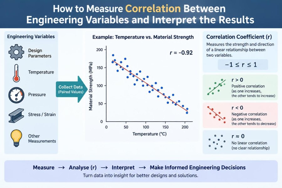
Correlation describes the direction and strength of association between two variables. If high values of one variable tend to occur alongside high values of another, the relationship is positive. If high values of one tend to occur alongside low values of the other, it is negative.
Correlation does not directly measure physical causation. It measures a pattern in observed data: how two quantities vary together across a set of measurements.
For example, pump flow rate and pressure drop may show a positive correlation over a particular operating range. That is a useful observation, but the engineering explanation still requires fluid mechanics, knowledge of the system layout, and checks for changing valve positions or operating conditions.
🧭 Positive, Negative, and Near-Zero Patterns
A correlation coefficient is commonly represented by r and lies between −1 and +1. Its sign gives the direction of the observed association.
| Value or pattern | Plain-language interpretation | Illustrative engineering example |
|---|---|---|
| Positive, r > 0 | Variables tend to increase together | Load torque and motor current |
| Negative, r < 0 | One variable tends to decrease as the other increases | Heat-sink temperature difference and cooling margin |
| Near zero, r ≈ 0 | No clear linear association | Part serial number and measured stiffness |
The magnitude indicates how closely the points follow a straight-line trend, not whether the result is good, bad, causal, or operationally important.
📏 Why Engineers Use Correlation
Engineering work often begins with more measured signals than clear explanations. Correlation provides a compact first screen for identifying variables worth investigating further.
It can help teams find candidate drivers of energy use, identify sensor channels that move unexpectedly together, compare quality metrics with process settings, and select inputs for predictive models. It is especially useful during exploratory analysis, when the goal is to reduce a large data set into questions that engineering knowledge can answer.
Used carefully, correlation saves time. Used alone, it can send an investigation in the wrong direction.
🧮 The Pearson Correlation Coefficient
The most familiar measure is the Pearson product-moment correlation coefficient. It measures the strength of a linear relationship: a relationship reasonably represented by a straight line.
For paired observations (xᵢ, yᵢ), Pearson’s coefficient is:
r = Σ[(xᵢ − x̄)(yᵢ − ȳ)] / √[Σ(xᵢ − x̄)² Σ(yᵢ − ȳ)²]Here, x̄ and ȳ are the sample means. The numerator captures whether deviations from the means tend to have the same sign or opposite signs. The denominator scales the result so it remains between −1 and +1.
You rarely need to calculate this by hand in practice, but understanding its structure matters: Pearson correlation is based on deviations around the average and is sensitive to unusually extreme measurements.
🧠 A Simple Intuition for the Formula
Imagine marking each measurement as above or below its usual value. When motor current is above average at the same times that torque is above average, their paired deviations have the same sign. Those products are positive and push r upward.
If current is above average when torque is below average, the products are negative and push r downward. If the pairings are mixed without a consistent pattern, positive and negative contributions tend to cancel.
This also explains why changing units does not change Pearson correlation. Converting pressure from kilopascals to pascals rescales values, but it does not change the underlying pattern of above- and below-average observations.
📊 Start with a Scatter Plot, Not a Coefficient
A scatter plot places one variable on the horizontal axis and the other on the vertical axis. Each point represents one paired observation. Before trusting any coefficient, look at this plot.
A single number can conceal a curved trend, separate operating clusters, a saturation limit, or one bad sensor reading. A scatter plot shows whether a linear summary is appropriate in the first place.
For a hypothetical heat-exchanger data set, outlet temperature may decline rapidly as flow first increases, then level off. Pearson r may describe some overall tendency, yet the actual engineering relationship is nonlinear and governed by heat-transfer behavior.
🗂️ Define the Question Before Collecting Data
“Are these variables correlated?” is often too broad. Define the physical and operational question first: Does bearing temperature increase with radial load at constant speed? Does dimensional variation change with cure temperature after accounting for batch?
A focused question determines what to measure, which variables to hold approximately constant, and which records should be compared. It also prevents an attractive but irrelevant correlation from becoming the main story.
State the expected mechanism before viewing results where possible. This does not guarantee that the expectation is correct, but it makes interpretation more disciplined.
⏱️ Pair Observations at the Same Meaningful Time
Every correlation calculation requires paired values. In time-series data, the pairs must represent the same physical moment or a physically meaningful delay.
A temperature sensor sampled every minute and a vibration sensor sampled every second cannot simply be placed side by side row by row. Resample, aggregate, or align the data with a documented method. Also account for process lag: a thermal response may follow a power change several minutes later.
Misalignment can weaken a real relationship or create a misleading one. For dynamic systems, correlation at zero time lag is only one part of the analysis.
🧹 Clean Data Without Hiding the Process
Remove or flag clearly invalid values, such as a disconnected sensor’s fixed error code or readings recorded during known equipment shutdowns. Keep a record of what was excluded and why.
Do not delete points merely because they disagree with the expected trend. An apparent outlier may be an instrumentation fault, but it may also reveal a distinct operating state, an emerging failure, or a previously overlooked input.
Useful checks include missing values, duplicated timestamps, inconsistent units, impossible ranges, calibration changes, and changes in sensor location. Data cleaning is an engineering activity, not just spreadsheet housekeeping.
🎯 Check Measurement Quality First
No statistical method can recover a relationship that has been buried under poor measurements. Sensor noise, quantization, drift, incorrect calibration, and inconsistent sampling all affect the observed correlation.
Random measurement noise generally weakens an observed association because it adds variation unrelated to the underlying process. Systematic error can be more troublesome: a shared temperature effect on two sensors may create an association that belongs to the instruments rather than the system.
Before interpreting small differences in coefficients, ask whether the measurement uncertainty is large enough to make those differences practically meaningless.
📐 Choose Pearson Correlation for Linear Patterns
Pearson correlation is a strong default when the scatter plot is roughly linear, observations are meaningfully paired, and a small number of extreme points do not dominate the result.
It is often appropriate for variables such as force and elastic displacement within a material’s linear range, or voltage and current for a resistive element under stable conditions. Even then, a high coefficient does not replace checks for changing conditions or shared inputs.
Pearson correlation is not a universal “relationship score.” Its purpose is specific: quantify linear co-variation.
🏷️ Use Spearman Correlation for Ranked Trends
Spearman rank correlation first replaces values with their ranks, then evaluates how consistently the ranks move together. It is useful when a relationship is monotonic: it consistently rises or falls, even if it is not a straight line.
For example, increasing surface roughness may be associated with increasing friction in a consistently ordered but nonlinear manner. Spearman correlation can reflect that ordered trend better than Pearson correlation.
It is also less sensitive than Pearson correlation to certain extreme values, though it is not immune to poor data or confounding. Tied values, common in rounded sensor readings, require appropriate handling by the software.
🪜 Know When Kendall’s Tau Helps
Kendall’s tau is another rank-based measure. It assesses whether pairs of observations are ordered consistently, using concordant and discordant pairs.
It can be helpful for smaller samples, ordinal assessments, and data with many ties, such as inspection ratings or ranked surface-quality categories. Its numerical values are not directly interchangeable with Pearson or Spearman values, so compare like with like.
For continuous process measurements, Pearson or Spearman is more commonly used as an initial descriptive tool. Kendall’s tau becomes particularly useful when ranking itself is the natural language of the data.
🌙 Nonlinear Relationships Can Look Uncorrelated
A correlation near zero does not prove that variables are unrelated. It only indicates little or no linear association for Pearson correlation.
Consider a hypothetical shaft system where vibration amplitude is lowest at a target speed and increases when speed is either lower or higher. The scatter plot forms a U-shape. Because positive and negative slopes occur on opposite sides of the minimum, Pearson r can be close to zero despite a strong operational relationship.
Plots, engineering models, transformations, and nonlinear regression are better tools for such patterns. Never let a single near-zero coefficient end an investigation prematurely.
🔢 What Counts as a Strong Correlation?
There is no universal threshold for “strong.” A coefficient’s practical meaning depends on sensor quality, process variability, sample size, operating range, and the consequence of acting on the result.
In a tightly controlled laboratory experiment, a modest correlation may signal an important physical effect. In a noisy plant-wide data set, a larger correlation may still be too weak for reliable prediction. Context matters more than a generic label.
Describe both the number and the visible pattern: “a moderate positive linear association over the tested load range” is more informative than calling a result simply strong.
🧩 Correlation Is Not Causation
Two variables can correlate because one affects the other, because the reverse is true, because both respond to a third variable, or because the pattern occurred by chance in the available sample.
Suppose compressor power and discharge temperature rise together. Power may contribute to heating, but both may also increase because demand raises compressor loading. The correlation alone cannot distinguish these mechanisms.
Establishing causation requires physical reasoning and, where feasible, controlled changes, experiments, validated models, or designs that account for alternative explanations.
🎛️ Watch for Confounding Variables
A confounder is a variable that influences both quantities being compared. It can create, weaken, or reverse an apparent association.
Ambient temperature, production rate, machine speed, product grade, and operator shift are common confounders in engineering data. For example, energy consumption and defect count may correlate simply because both rise when production volume rises.
Plot data by operating condition, analyze stable subsets, or include the likely confounder in a multivariable model. Asking “what could drive both?” is one of the most valuable habits in correlation analysis.
🏭 Separate Operating Regimes
Many systems do not behave as one population. A turbine at startup, steady load, and shutdown may follow different relationships, as may a production line making different products.
Combining all regimes can yield a coefficient that describes none of them well. A positive overall correlation may disappear within each operating mode, or separate clusters may indicate different physical states.
Use operating flags, setpoints, product identifiers, or time intervals to segment data. Then compare scatter plots and coefficients within each meaningful regime.
🧪 Use Controlled Experiments When Decisions Matter
Observational data are valuable, but deliberate experiments provide stronger evidence when it is safe and practical to run them. Change one controllable factor through a planned range while holding major alternatives stable or recording them carefully.
Randomizing test order can reduce the risk that time-related drift is mistaken for an effect. Repeating runs helps show whether the observed relationship is stable rather than a one-off result.
For complex systems, a designed experiment may reveal interactions that pairwise correlation cannot show. The goal is not merely a higher coefficient; it is a defensible understanding of which factors influence the response.
📉 Understand the Coefficient of Determination
For a simple linear regression with one predictor and an intercept, squaring Pearson’s correlation gives R², the coefficient of determination. It describes the proportion of variation in the response accounted for by that fitted linear model in the sample.
If r is negative, R² is still positive because the sign is removed. That means R² loses the direction of the relationship, so report the slope or correlation sign as well.
R² is often misread as proof that a model is correct or causal. It is neither. It is a measure of fit for a specified model and data set, and it should be considered alongside residual plots and engineering plausibility.
📈 Regression Answers a Different Question
Correlation treats the two variables symmetrically. Regression does not: it models a response variable as changing with one or more input variables.
Use correlation when asking whether temperature and vibration move together. Use regression when asking how vibration might be estimated from temperature, speed, load, and other inputs, with an explicit model and residual error.
A high correlation does not automatically make a good predictive model. Prediction requires validation on data not used to fit the model, attention to future operating conditions, and a realistic treatment of uncertainty.
🕰️ Time-Series Data Need Extra Caution
Measurements collected over time are often autocorrelated: a value resembles the previous value because the physical system has inertia. Two unrelated signals can also trend together over time, producing a misleading correlation.
For instance, two temperatures may both rise during a warm-up period even if neither directly influences the other. Examine trends, differences, lags, and process phases rather than correlating long raw traces without context.
Lagged correlation can explore whether one signal consistently precedes another, but it remains descriptive. A lag pattern may reflect transport delay, control-loop behavior, or a common scheduled change.
🔁 Cross-Correlation Can Reveal Possible Delays
Cross-correlation calculates association after shifting one time series relative to another. It can help estimate a plausible delay between an input and a response.
In a heating process, electrical power may change first and a downstream temperature sensor may respond later. A peak at a positive or negative lag, depending on the chosen convention, can guide investigation of that delay.
Use consistent sampling, remove obvious trends where appropriate, and interpret results with process knowledge. Feedback control can make delays and associations difficult to interpret because controller actions respond to the very measurements being analyzed.
🧷 Outliers Can Change the Story
Pearson correlation is sensitive to outliers because distant points have large deviations from the mean. One erroneous high-pressure reading paired with a high-flow event can noticeably alter the coefficient.
Inspect influential points individually. Verify units, timestamps, instrument condition, and operating notes before deciding whether a point is erroneous, exceptional, or valid.
Report analyses with and without clearly documented invalid points when that comparison materially changes the conclusion. If valid extremes are part of normal operation, excluding them may produce a deceptively tidy result.
🧊 Restricted Range Can Hide a Real Effect
Correlation depends on the range of values observed. If all tests are run at almost the same load, there may be too little variation to reveal the relationship between load and deflection.
This is called range restriction. A low coefficient from a narrow operating window does not necessarily contradict a well-established relationship across the full design range.
When planning tests, choose a safe, relevant range that spans the conditions needed for the decision. Then state clearly which range the conclusion applies to.
🧾 Statistical Significance Is Not Practical Significance
A statistical test can assess whether an observed correlation would be unusual under a particular no-association model. The resulting p-value depends heavily on sample size and assumptions about the data.
With many observations, a very small association may be statistically detectable but too weak to matter operationally. With few observations, a potentially important relationship may remain uncertain.
Pair any significance assessment with effect size, confidence intervals where appropriate, plots, measurement uncertainty, and the practical consequence of a wrong decision. Statistical output should inform judgment, not replace it.
🧑💻 Calculate Correlation in Everyday Tools
Spreadsheets, numerical software, and programming languages can calculate correlation quickly. The harder part is ensuring that the selected rows, units, timestamps, and filters represent the question you intend to answer.
A practical workflow is:
- Export paired measurements with clear variable names and units.
- Check missing values, timing alignment, and known invalid states.
- Create a scatter plot before calculating a coefficient.
- Compute Pearson or rank correlation suited to the pattern.
- Segment by operating regime and repeat when justified.
- Document exclusions, transformations, and interpretation.
In a spreadsheet, verify that the formula ranges are identical in length and do not include headers or mismatched blank cells. Quiet range errors can produce a number that looks credible but compares the wrong observations.
🧱 Build a Correlation Matrix Carefully
A correlation matrix lists the pairwise correlations among several variables. It is useful for quickly scanning a large set of channels, such as pressures, temperatures, currents, and quality measures.
However, a matrix can encourage data fishing: with many pairs examined, some large-looking values may occur without a meaningful mechanism. It also hides shape, time order, and operating clusters.
Use the matrix to prioritize plots and engineering questions, not as a final explanation. For model inputs, remember that highly correlated predictors can create multicollinearity, making individual regression coefficients unstable or difficult to interpret.
🛠️ A Worked Hypothetical Example
Imagine a maintenance engineer investigating a fan. During steady production, they collect synchronized motor current and vibration readings at several load levels. The scatter plot slopes upward, and Pearson correlation is positive.
The first conclusion is modest: within the sampled steady-production conditions, higher current tended to occur with higher vibration. The engineer then checks speed, damper position, bearing temperature, and whether the pattern remains after separating product types.
If vibration still rises with current at comparable speed and damper position, the relationship becomes more informative. It may reflect increased aerodynamic loading, but it still does not diagnose bearing damage by itself. Inspection history, spectral vibration analysis, and equipment design data are needed for that claim.
🚫 Common Interpretation Mistakes
- Treating correlation as proof of cause: always consider reverse causation and shared drivers.
- Ignoring a scatter plot: a coefficient cannot reveal curves, clusters, or sensor failures.
- Mixing operating states: startup, shutdown, and steady production often need separate analysis.
- Using a universal strength label: practical meaning depends on the system and decision.
- Forgetting time lag: a real response may occur after the proposed input changes.
- Testing every pair without a question: more comparisons increase the chance of misleading patterns.
Most of these mistakes are avoided by combining statistics with a process diagram, operating records, and basic physical reasoning.
📝 Report Results So Others Can Evaluate Them
A useful correlation report gives enough context for another engineer to understand what was compared and where the conclusion applies. Do not report only “r = 0.72.”
Include the variables and units, sample size, time period or test condition, correlation type, any lag used, handling of missing or invalid data, operating regime, and an accompanying scatter plot. Describe the result in careful language that distinguishes association from cause.
For example: “During stable operation at the tested settings, flow rate and pressure drop showed a positive approximately linear association. This observation is consistent with expected system resistance but does not isolate the effects of valve position and fluid temperature.”
✅ The Core Principle: Use Correlation as Evidence, Not a Verdict
Correlation is most valuable when it starts a better engineering question. It summarizes a visible pattern, helps identify variables for closer study, and can support monitoring or model development when its limitations are respected.
Good practice follows a sequence: define the physical question, verify data quality and timing, visualize the measurements, choose a suitable coefficient, check confounders and operating regimes, then interpret the result against engineering knowledge.
The key distinction is simple: a correlation coefficient describes how variables behaved together in the data you observed. A reliable engineering conclusion requires evidence about why they behaved that way and whether the pattern will hold where you intend to use it.
Measure the pattern, inspect the context, and let physics guide the conclusion—not the coefficient alone. 📐📊🔧